
Linear-upper-coverage Smoothing for Peak Finding
by lucainiaoge
Intro
I came up with this idea on October 9th, 2020, when I was considering how to find the overtone peaks in a spectrogram. I happened to be playing LIMBO the previous day, and that inspired me to come up with my idea regarding Linear-upper-coverage (LUC), which converts the peak finding problem into linear optimization subtasks.
- It is recommended that readers have grasped basic knowledge about calculus, convex optimization and digital signal processing (DSP). Still, if those pre-requisites are not satisfied, it is also OK to understand my ideas and algorithms. Most of those knowledges are helpful when readers want to understand my proofs for the Lemmas or Theorems proposed in this article.
- If [Math Processing Error] occurs or figures are not showing, please refresh this page or switch to another browser (Google chrome is recommended).
- One more tip: this article is a little bit long. However, if you skip my rationales/proofs and go directly to my motivations and experiment results, you will finish reading this article quicker. Anyway, welcome to delve into my math works and logics in order to understand LUC deeply, and welcome to correct me if I made mistakes.
Problem Definition and Motivation
The Problem
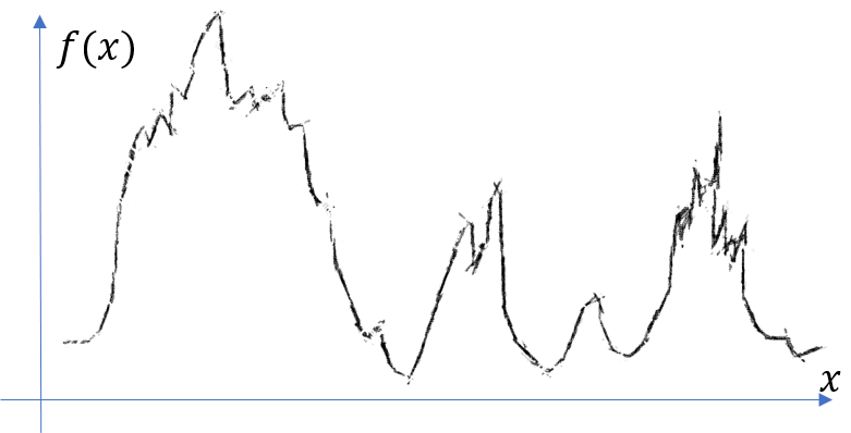
How to find the peaks in the following curve?
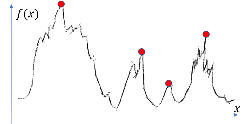
If we manually mark the peaks, the result may normally look like the following figure?
However, how to design an algorithm to robustly find the desired peaks (local maxima)?
To answer this question, we have to ask ourselves: what is a desired peak?
If we just want every local maxima, we may get this following result:
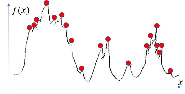
And according to our current definition of “desired peak”, this ugly result is correct.
Therefore, you may be willing to design an algorithm which is adaptable according to our variable definitions for a “desired peak”.
What Inspired Me
Well, in addition to the inspiring peak-finding-problem itself, another incentive of my idea is a rolling wheel on a coarse road:
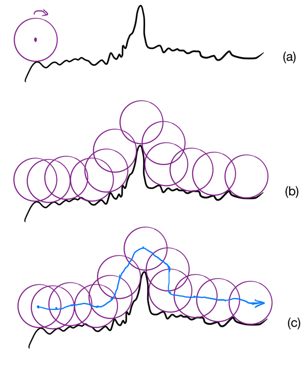
As you can see: the centroid of the wheels form up a much smoother curve (although still a little bumping) than the original curve. However, several insignificant local maxima are still troublesome. And it is also a little bit hart do model a wheel rolling on a coarse road with a few lines of codes. So how to improve this idea?
I was lucky to be playing LIMBO the previous day, and one scene in the vedio game LIMBO just struck me:
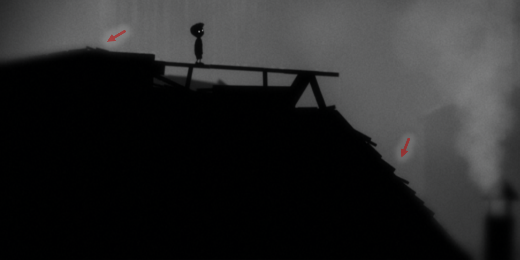
Notice the the red arrows: there are tiles covering the roof/hill (whatever it looks like as it is dark).
So, why not cover our curve with tiles? I drew the following picture to show my idea of tile-covering:
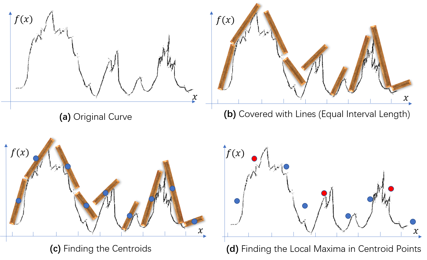
First, divide the x-axis into intervals; second, cover the curves in each intervals with tiles; third, find the centroid of each tile; finally, use the centroid scatters to find the local maxima.
Notice that we can cover over curve with tiles of different lengths, which is equivalent our variable definitions on “desired peak”: if we use short tiles, we will be more sensitive to small local maxima, while long tiles will ignore the local maxima which are insignificant in terms of a smaller measure on $x$.
Now comes the question: how to implement this idea?
From Peak Finding to Linear Optimization
Deriving the Basic Formulation
As the title of this section suggests, I utilized linear optimization to solve the problem. Among the four steps in the previous section, you may notice that the phrase “over the curves in each intervals with tiles” is not clearly defined. How can we cover a curve with a tile? Here is where linear optimization comes into being:
Suppose we got an interval $x \in [x_i,x_{i+1}]$, where a 1-D curve $f(x)$ is defined. The tile is depicted as $l_i(x)=a_i x+b_i$. Obviously, we must have $f(x) \leq l_i(x), \forall x \in [x_i,x_{i+1}]$. With this constraint, we want to find the parameters $(a_i,b_i)$ such that the tile seems to cover the curve.
Newton’s laws suggest: if you put an object in a gravitatio, it is stable when its gravitational potential energy reaches its minimum. If we assume that the density of our tiles is uniformly distributed, we can conclude that the tile’s gravitational potential energy can be calculated by a particle locating at its centroid, which is $(\frac{x_i+x_{i+1}}{2},l_i(\frac{x_i+x_{i+1}}{2}))$. Therefore, we get our objective function: $l_i(\frac{x_i+x_{i+1}}{2})=a_i\frac{x_i+x_{i+1}}{2}+b_i$.
To sum up, we get the linear optimization problems:
$\forall i=1,2,…$, solve the linear programming (LP)problem within interval $[x_i,x_{i+1}]$:
$$min_{a_i,b_i} \quad a_i\frac{x_i+x_{i+1}}{2}+b_i $$ $$s.t. f(x) \leq a_i x+b_i, \forall x \in [x_i,x_{i+1}]$$
And I may call it linear-upper-coverage (LUC) algorithm.
Notice that there are infinite constraints, which are intractable. One intuitive way is to sample the interval $x \in [x_i,x_{i+1}]$ to get $x_{i}^{k} \in [x_i,x_{i+1}], \forall k=1,2,…,K$. And consequently, the linear constraints become: $$f(x_{i}^{k}) \leq a_i x_{i}^{k}+b_i, \forall k=1,2,…,K$$
Until now, we are able to solve that linear optimization problem with inequality constraints! The classical linear programming algorithms (e.g. the Simplex Method) are well-equipped to sove them!
Formal LUC Definition Generalizing Interval Partitions
You may noticed that although I divided the x-axis equally, the lengths of tiles are not the same. Is it necessary to set the tile lengths all the same? This is actually about the choosing the segmentation strategy, i.e. the procedure to get $[x_i,x_{i+1}], i=1,2,…$
Therefore, if restricted to linear coverage, the most configurable aspect is the segmentation strategy. Not only can we segment in equal length, we can also segment in a log-scale, or even sample randomly. Different segmentation strategy lead to different definitions of “desired peak”.
Also, it is not necessary to assume that the intervals do not overlap. Instead, we can arbitrarily sample the curve and construct intervals for each of those sample points, even if those intervals can overlap. Such more general definition becomes:
Definition 1 (normal LUC): Given $f:D\rightarrow \pmb{R}$, sample data points $x_i\in D,i=1,2,…$. Define intervals $I_i = [x_i^l,x_i^r]$ where $x_i \in I_i$, and define linear segments $l_i(x)=a_i x+b_i, \forall x\in I_i$.
Define the linear programming problems $LUC_i$ within intervals
$$LUC_i:\quad min_{a_i,b_i} \quad l_i(\frac{1}{2}(x_i^l+x_i^r))$$ $$s.t. f(x) \leq l_i(x), \forall x \in I_i$$ The LUC solution is the set of all optimum linear segments, i.e. $l_i^{\star}(x)$
From now on, $x_i$ no longer means the left endpoint of interval $I_i$, but the centroid point of interval $I_i$. The left endpoint of interval $I_i$ is written as $x_i^l$ instead. (If I sometime breaks this law, please understand that because those cases are obvious.)
Moreover, we can cover the curve with actually whatever function we like: circles, ovels etc. I chose lines because they look more simple and intuitive. What about other elements? It might be worth trying, but I am not going to talk about them at this moment…
Proof that LUC Has Smooth Effects: Convex Case
If we want to prove that an algorithm can smoothify a curve, we have to prove that the algorithm dampens the high-frequency components in certain ways.
The main challenge to prove this for LUC is that there are linear-programming calculations in each interval, which is non-trivial. I find it difficult to prove this even convex constraint is considered.
Two Lemmas with Proof
I start from the (lower) convex segments defined in $[x^l,x^r]$:
$$f(\lambda x^l+(1-\lambda) x^r)\leq \lambda f(x^l)+(1-\lambda) f(x^r), \forall 0\leq \lambda \leq 1$$
Intuitively, we can reach the following conclusion:
Lemma 1 (LUC for convex function): if $f:[x^l,x^r]\rightarrow \pmb{R}$ is convex in $[x^l,x^r]$, then the optimum LUC function becomes $l^{\star}(x)=\frac{f(x^l)-f(x^r)}{x^l-x^r} (x-\frac{x^l+x^r}{2}) + \frac{f(x^l)+f(x^r)}{2}$
Proof:
①First prove that the given $l^{\star}$ obeys the constraints of LUC linear programming.
That constraint is: $f(x) \leq l(x), \forall x \in [x^l,x^r]$. If we apply $l^{\star}$ to that constraint, we just need to prove: $f(x) \leq l^{\star}(x), \forall x \in [x^l,x^r]$.
Plug in the convex assumption on $f(x)$ and we get: $f(\lambda x^l+(1-\lambda) x^r)\leq \lambda f(x^l)+(1-\lambda) f(x^r), \forall 0\leq \lambda \leq 1$.
As $f(x^l) \leq l^{\star}(x^l)$ and $f(x^r) \leq l^{\star}(x^r)$, we get $\lambda f(x^l)+(1-\lambda) f(x^r)\leq \lambda l^{\star}(x^l)+(1-\lambda) l^{\star}(x^r) = l^{\star}(\lambda x^l+(1-\lambda) x^r)$.
Therefore, we proved that $f(x) \leq l^{\star}(x), \forall x \in [x^l,x^r]$ is true.
②Then prove that $l^{\star}$ is the optimum.
Recall that the objective function is $l(\frac{x^l+x^r}{2}) = a_i\frac{x^l+x^r}{2}+b_i$.
If we want to decrease the objective value $l(\frac{x^l+x^r}{2})=\frac{l(x^l)+l(x^r)}{2}$, either $l(x^l)$ or $l(x^r)$ should be decreased.
However, according to the constraints, $f(x^l) \leq l(x^l)$ and $f(x^r) \leq l(x^r)$: once we have $f(x^l) = l^{\star}(x^l)$ and $f(x^r) = l^{\star}(x^r)$, we can assert that $l^{\star}$ reaches the optimum, for neither $l^{\star}(x^l)$ or $l^{\star}(x^r)$ can be decreased. □
On the other hand, if we assume that $f(x)$ is bounded in interval $[x^l,x^r]$, it is also intuitive to reach the following conclusion:
Lemma 2 (existance of LUC solutions and tightness): if $f:[x^l,x^r]\rightarrow \pmb{R}$ is bounded, then:
- There are at least two zero-slackness LUC constraints at $x^{-}$ and $x^{+}$ ($x^{-}\leq x^{+}$); the term zero-slackness indicates that $f(x^{-})=l^{\star}(x^{-})$ and $f(x^{+})=l^{\star}(x^{+})$.
- Equality of $x^{-}\leq x^{+}$ is reached only when $x^{-}=x^{+}=x^l$ or $x^{-}=x^{+}=x^r$
Proof:
① First prove that there is at least one optimum solution for the LUC problem.
As $f(x)$ is bounded in interval $[x^l,x^r]$, assume that $m<f(x)<M_1<M_2$, there exists $l(x)=a_i x+b_i$ such that $M_2>l(x^l)>M_1>f(\forall x)$ and $M_2>l(x^r)>M_1>f(\forall x)$. Therefore, feasible region is not empty.
On the other hand, there exists $l(x)=a_i x+b_i$ such that $m<f(x^l)\leq l(x^l)$ and $m<f(x^r)\leq l(x^r)$. This is to say, the objective $\frac{l(x^l)+l(x^r)}{2}>m$. Therefore, the objective cannot be arbitrarily small.
In sum, there is at least one optimum solution for the LUC problem.
② Then prove that the optimum solution lead to zero slackness. Recall the complementary slackness theorem:
Given a standard LP problem $$min\quad cx, \quad s.t. \quad Ax \geq b$$ and its dual problem $$max\quad b^T y, \quad s.t. \quad A^T y \leq c^T$$ Definition of slackness of the $k^{th}$ constraint is $s_k = A_k x - b_k$.
The complementary slackness theorem says that if a feasible solution $x_0$ is optimum (which exists because of ①), and its corresponding dual solution is $y_0$ is also optimum, then $x_0^T (c-A^T y_0)=0$ and $y_0^T (A x_0 - b)=0$.
Therefore, for those $y_0^k \neq 0$, we must have $A_k x_0 - b_k = 0, k \in \lbrace k:y_0^k \neq 0 \rbrace$. As a result, $s_k = A_k x_0 - b_k = 0,k \in \lbrace k:y_0^k \neq 0 \rbrace$.
Translate this into LUC context: $x_0=(a_{i}^{\star},b_{i}^{\star})$, $A=[x^{[1:K]},ones(1,K)^T]$, $c=[\frac{x^l+x^r}{2},1]$ and $b=[f(x^1),…,f(x^K)]^T$. The “$y_0^k$” in LUC cannot be all zero, or otherwize $c=0$, which is not true. Therefore, there always exists $k$ such that “$A_k x_0 - b_k = 0$”, which is actually $f(x^k)=l^{\star}(x^k)$ (the $k^{th}$ constraint), leading to zero slackness.
③ Then prove that there are at least two different tight constraints.
According to the convexity of linear feasible region (which is a polyhedron), the optimum solution touches the vertex of that region. As we know, the vertex of a region is an intersection of two hyperplanes (in LUC, they are actually two 2-D lines, because there are only two variables), corresponding to two different constraints. Therefore, if there are at least two constraints which have zero slackness, they are different.
④ Finally prove the property when $x^{-}=x^{+}$.
We know that each constraint can be linked with an $x$ in $[x^l,x^r]$. Moreover, the statement $x\in [x^l,x^r]$ indicates two more underlying constraints $x\geq x^l$ and $x\leq x^r$. Recall ③: the two constraints at $x=x^{-}$ and $x=x^{+}$ are different. If a constraint at $x=x^{-}$ is tight and $x^{-}=x^{+}$, then this case only happens at $x=x^l$ or $x=x^r$, because: any $x\in (x^l,x^r)$ can be linked with only one constraint $f(x)\leq l(x)$; but at $x=x^l$, there exists one more constraint $x\geq x^l$, which reaches tightness (and the case when $x=x^r$ is similar). In conclusion, the statement $x^{-}=x^{+}$ indicates that two tight constraints sharing the same point, and such case can only happen at $x=x^l$ or $x=x^r$; consequently, $x^{-}=x^{+}=x^l$ or $x^{-}=x^{+}=x^r$.□
Explore the Effects of LUC on DTFT Spectrum
Now, we have all the ingradients! What is left is to describe our problem in a proper way. Consider a uniformally-sampled sequence of $f(x)$, which is written as $[f_i] = [f_1,f_2,…] = [f(x_1),f(x_2),…]$.
Without downsampling, we do LUC for each interval centered with the $i^{th}$ point, i.e. the interval $[x_i-\Delta x,x_i+\Delta x]$. It is also OK to write this interval as $[x_{i-\Delta i},x_{i+\Delta i}]$ because of equal-partition.
Therefore, we have the LUC problem formally:
$$min_{a_i,b_i} \quad a_i x_i+b_i $$ $$s.t. f(x) \leq a_i x+b_i, \forall x \in [x_{i-\Delta i},x_{i+\Delta i}]$$
According to Lemma 2, there are at least two points $x_i^{-}$ and $x_i^{+}$ such that $f(x_i^{-})=l_i^{\star}(x_i^{-})$ and $f(x_i^{+})=l_i^{\star}(x_i^{+})$. We can subsequently determine $l_i^{\star}$ with those two points: $$a_i^{\star} = \frac{f(x_i^{-})-f(x_i^{+})}{x_i^{-}-x_i^{+}}$$ $$l_i^{\star}(x) = a_i^{\star}(x-\frac{x_i^{-}+x_i^{+}}{2})+\frac{f(x_i^{-})+f(x_i^{+})}{2} \quad (*)$$
Consequently, I write the LUC version of uniformally-sampled sequence as $[f_i^{\star}] = [f_1^{\star},f_2^{\star},…] = [l_1^{\star}(x_1),l_2^{\star}(x_2),…]$
Assume that $f(x)$ is convex in each interval $[x_{i-\Delta i},x_{i+\Delta i}]$ (no need to be convex in the overall definition interval). Then calculate the DTFT for both $[f_i]$ and $[f_i^{\star}]$:
$$F(\omega) = {\rm DTFT}[f_i] = \sum_i f_i e^{\sqrt{-1}\omega i} \quad ①$$ $$F^{\star}(\omega) = {\rm DTFT}[f_i^{\star}] = \sum_i f_i^{\star} e^{\sqrt{-1}\omega i} = \sum_i [a_i^{\star}(x_i-\frac{x_i^{-}+x_i^{+}}{2})+\frac{f(x_i^{-})+f(x_i^{+})}{2}] e^{\sqrt{-1}\omega i} \quad ②$$
According to the convexity assumption, we can apply Lemma 1, which says that $l_i^{\star}(x)=\frac{f(x_{i-\Delta i})-f(x_{i+\Delta i})}{x_{i-\Delta i}-x_{i+\Delta i}} (x-\frac{x_{i-\Delta i}+x_{i+\Delta i}}{2}) + \frac{f(x_{i-\Delta i})+f(x_{i+\Delta i})}{2}$
Compare this with $(*)$ and we will get $x_i^{-}=x_{i-\Delta i}$ and $x_i^{+}=x_{i+\Delta i}$.
Plug this conclusion into $②$ and also apply the equality that $x_i = \frac{f(x_{i-\Delta i})+f(x_{i+\Delta i})}{2}$, we will get:
$F^{\star}(\omega) = {\rm DTFT}[f_i^{\star}] = \sum_i \frac{f(x_{i-\Delta i})+f(x_{i+\Delta i})}{2} e^{\sqrt{-1}\omega i}$
$= \sum_i \frac{f_{i-\Delta i}+f_{i+\Delta i}}{2} e^{\sqrt{-1}\omega i}$
$= \frac{1}{2}({\rm DTFT}[f_{i-\Delta i}] + {\rm DTFT}[f_{i+\Delta i}])\quad ③$
We know that ${\rm DTFT}[f_{i-\Delta i}]=\sum_i f_{i-\Delta i}e^{\sqrt{-1}\omega i}=\sum_i f_{i}e^{\sqrt{-1}\omega (i+\Delta i)}=e^{\sqrt{-1}\omega \Delta i}\sum_i f_{i}e^{\sqrt{-1}\omega i}=e^{\sqrt{-1}\omega \Delta i}{\rm DTFT}[f_{i}]$
Therefore, $③$ becomes $$F^{\star}(\omega) = {\rm DTFT}[f_i^{\star}] = \frac{1}{2}[e^{\sqrt{-1}\omega \Delta i}+e^{-\sqrt{-1}\omega \Delta i}]F(\omega) = F(\omega){\rm cos}(\omega \Delta i) \quad ④$$
Finally, we can reach from $④$ that $\vert F^{\star}(\omega) \vert = \vert F(\omega)\vert \vert {\rm cos}(\omega \Delta i)\vert \leq \vert F(\omega)\vert$
Summing up the discussions above:
Theorem 1 (smooth effect of convex LUC): given $\Delta i > 0$ and bounded $f(x):D\rightarrow R$, sample a sequence $x_i, i=1,2,…$ from $D$, whose corresponding intervals are $[x_{i-\Delta i},x_{i+\Delta i}], i=1,2,…$; the LUC centroids form a sequence $f_i^{\star}=l_i^{\star}(x_i), i=1,2,…$ whose DTFT is $F^{\star}(\omega)$, while the sampled curve becomes $f_i=f(x_i), i=1,2,…$ whose DTFT is $F(\omega)$. Then we have:
if $f(x)$ is convex in intervals $[x_{i-\Delta i},x_{i+\Delta i}], i=1,2,…$ separately, then $F^{\star}(\omega)=F(\omega){\rm cos}(\omega \Delta i)$
Due to Taylor’s approximation of ${\rm cos}(\omega \Delta i)$: when $\omega$ is near zero, $F^{\star}(\omega)$ is near $F(\omega)$; but when $\omega$ is a little bit far from zero, $F^{\star}(\omega)$ will be dampened. Of course, the choice of $\Delta i$ is also a factor controlling such influence.
To understand this effect more intuitively, here is an example, in which $\Delta i = 1/2$, and $f(x)$ is convex in every separate interval.
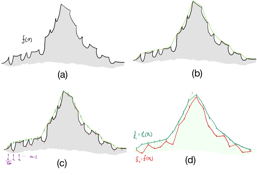
The red line (downsampled results) is more rugged than the green line (LUC centroids), which confers to my previous analysis.
A Candidate-set LUC Algorithm for General Cases
In the previous section, we discussed the LUC for a convex segment. More importantly, we proved Lemma 2, which guarentees the existance of solution, and even gives the exact solution: $$a_i^{\star} = \frac{f(x_i^{-})-f(x_i^{+})}{x_i^{-}-x_i^{+}}$$ $$l_i^{\star}(x) = a_i^{\star}(x-\frac{x_i^{-}+x_i^{+}}{2})+\frac{f(x_i^{-})+f(x_i^{+})}{2} \quad (*)$$
But it did not touch the essencial case of the tile covering a rugged curve whose convexity is ill defined. How to get a more clear mind about the rugged case? My plan is to find candidates in that rugged curve, from which we select two of them as $x_i^{-}$ and $x_i^{+}$ to determine our final result.
Before delving into this, we look at several examples…
Intuitive Examples
There are different curves and we will cover each of those with a line.
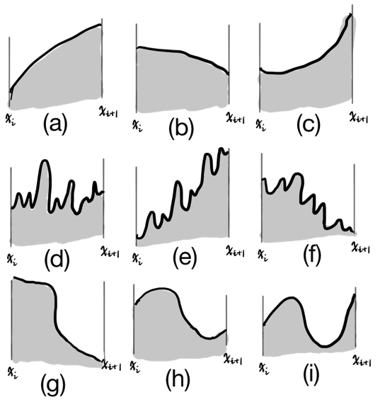
Case (c) is a convex, whose solution is that its $x_i^{-}$ and $x_i^{+}$ are actually the endpoints, which has already been proven.
Case (a) and (b) are concave cases, which are intuitively different from the convex case.
Case (d),(e) and (f) are rugged cases.
Case (g),(h) and (i) are combinitions of convex and concave segments. (h) and (i) has local maxinima, while (g) is monotonic.
Think for a while about the results…
And then, I give my intuitions:
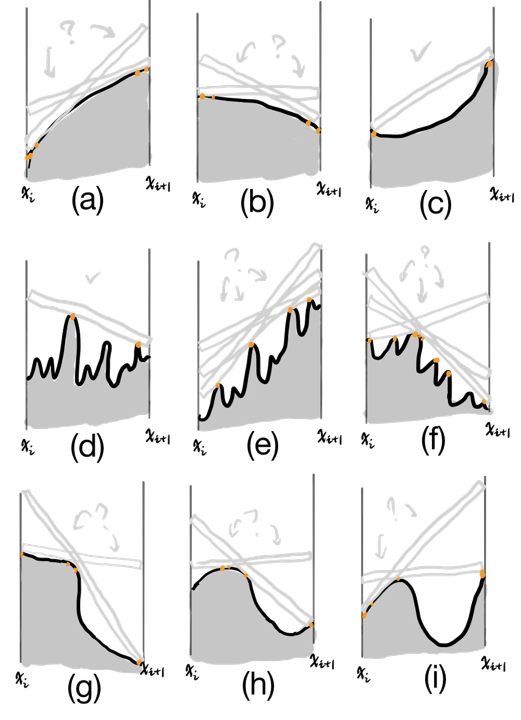
My finding is that: the candidate points (marked in orange) are such typical points:
- The local maximima
- The endpoints $X^l=(x^l,f(x^l))$ and $X^r=(x^r,f(x^r))$
- The curve point $P$ such that the slope of $PX^l$ reaches maximum; the curve point $Q$ such that the slope of $QX^r$ reaches minimum
Designing Candidate-Set Algorithm
My intuition leads to an algorithm to find the candidate points:
First, deal with the problem of finding local maximima:
Algorithm 1 (finding local maxima): $m=locmax(y)$
(1-based indexing is used) Given sample squence $y = [y_1,y_2,…,y_k,…,y_K]_{1\times K}$
- initialize a buffer $b = [1,0,…,0,…,0,0]_{1\times (K+1)}$
- initialize the result $m = [0,0,…,0,…,0]_{1\times K}$
- for $k=1,2,…,K-1$:
- $\quad$ $b[k+1] = bool(y[k] \geq y[k+1])$
- for $k=1,2,…,K$:
- $\quad$ $m[k] = b[k]·\overline{b[k+1]}$
- return $m$
Then, deal with the problem of finding $P$ and $Q$:
Algorithm 2 (finding $P$ and $Q$): $k_P,k_Q=findPQ(x,y)$
(1-based indexing is used) Given sample squence $y_{1:K}$ and its corresponding x-axis $x_{1:K}$
- $p = (y[2:K]-y[1])/(x[2:K]-x[1])$
- $q = (y[1:K-1]-y[K])/(x[1:K-1]-x[K])$
- $k_P = {\rm argmax}_k p[k]$
- $k_Q = 1+{\rm argmin}_k q[k]$
- return $k_P,k_Q$
Next, we reach the algorithm for getting the candidate set:
Algorithm 3 (finding candidate set): $I_c=findCandidate(x,y)$
(1-based indexing is used) Given sample squence $y_{1:K}$ and its corresponding x-axis $x_{1:K}$
- initialize $I_c = \lbrace 1,K \rbrace$
- $m=locmax(y)$
- $I_m = find(m==1)$
- $k_P,k_Q=findPQ(x,y)$
- $I_c = I_c \cup I_m \cup \lbrace k_P,k_Q \rbrace$
- return $I_c$
Now, take a look at the example (d),(e) and (f) in the last section: as those curves are rugged, the candidate points in $\lbrace (x_{i_c},x_{i_c}): i_c \in I_c \rbrace$ still form a rugged curve. Why not plug those points again into Algorithm 3? Consequently, we get $\hat{I_c}=findCandidate(x[I_c],y[I_c])$, as illustrated in the following figure:
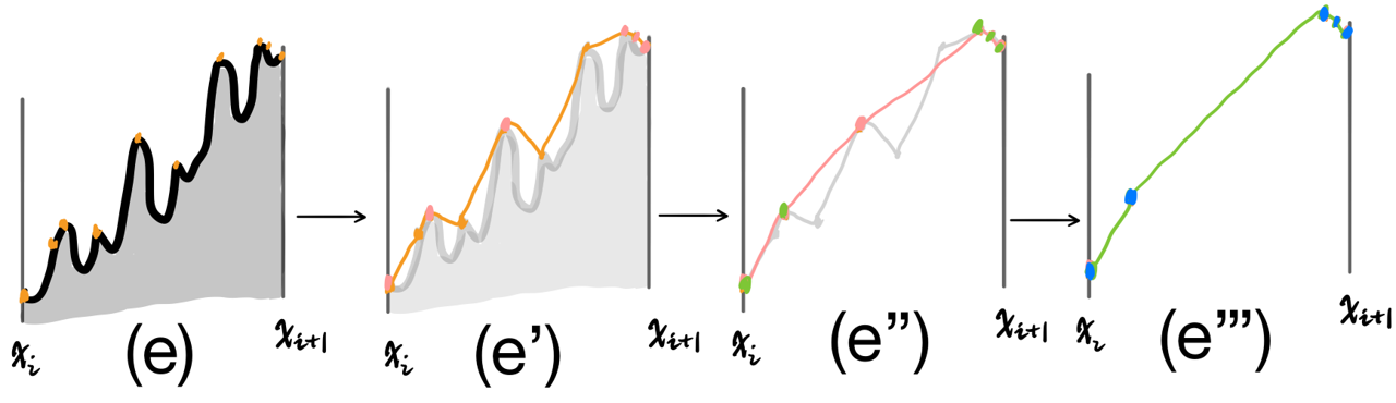
This leads to the ultimate algorithm:
Algorithm 4 (finding the smallest candidate set): $I_c=findCandidateSmallest(x,y,N)$
(1-based indexing is used) Given sample squence $y_{1:K}$ and its corresponding x-axis $x_{1:K}$;
$N$ denotes the max iteration times;
- initialize $I_c = \lbrace 1,2,…,K \rbrace, \tilde{I}=I_c, \hat{x} = x[I_c], \hat{y} = y[I_c]$
- for $n$ in $range(N)$:
- $\quad$ $\hat{I_c}=findCandidate(\hat{x},\hat{y})$
- $\quad$ if $\vert \hat{I_c} \vert == \vert I_c \vert$:
- $\quad\quad$ break
- $\quad$ else:
- $\quad\quad$ $I_c=\hat{I_c}$
- $\quad\quad$ $\tilde{I} = \tilde{I}[I_c], \hat{x} = \hat{x}[I_c], \hat{y} = \hat{y}[I_c]$
- return $\tilde{I}$
Finally, we reduce the number of constraints to those indexed by $I_c$.
Reflections
Why does the candidate-set algorithm work? Obviously, my intuitive explanations are far from compelling. To develop the following sections and to reconcile the effectiveness of candidat-set algorithm, I need to introduce my hypothesis, which is not proved at this moment:
Hypothesis 1 (equivalence of candidate-set in terms of LUC):
if the candidate set for bounded $f(x):I_i\rightarrow R$ is $I_{ci}$, then the normal LUC problem reduce to: $$LUC_i:\quad min_{a_i,b_i} \quad l_i(x_i)$$ $$s.t. f(x) \leq l_i(x), \forall x \in I_{ci}$$
Or in the language of Lemma 2: $x_i^{-}\in I_{ci}$ and $x_i^{+}\in I_{ci}$
In addition, if you are careful enough, you may find that my definition for candidate-set is flawwed: it does not lead to the equivalent result as the normal LUC. This can be proven by the figure in the previous section which illustrates the candidate-set algorithm, which provides a counter-example: the ultimate LUC calculated based on the blue points actually violates the LUC constraints based on the initial black curve!
Luckily, although this effect sometimes happens, the LUC results do not seriously change. I am going to demonstrate this in the experiment section.
Still, I have my solution which can perfectly solve this flawwed-definition problem. The key is: modify the $3^{rd}$ criterion to get a tentative $4^{th}$ criterion:
- For type 1 candidate points $X_k = (x_k,f(x_k))$ (which are local maxima), find curve points $P_k = (x_{k}^{+},f(x_{k}^{+})),Q_k = (x_{k}^{-},f(x_{k}^{-}))$ for each $X_k$, such that
- $x_{k}^{+}>x_k$ and the slope of $X_k P_k$ reaches maximum
- $x_{k}^{-}<x_k$ and the slope of $Q_k X_k$ reaches minimum
Consequently, the candidate-set finder algorithm should be modified according to the $4^{th}$ criterion. Fortunatelly, it is quite easy by changing Algorithm 2 and 3 a little bit. After all, I am going summarize all about candidate-set algorithm in the next section.
Formal Definition for Candidate-set Algorithm
Definition 2 (full definition for candidate set): Given bounded $f(x):I\rightarrow R$;the endpoints are $x^l=inf(I),x^r=sup(I)$.
Then, the candidate set for $I$ is written as $I_{c}=\lbrace x:x\in I_m, x\in I_{e}, x\in I_{e}^a, x\in I_{m}^a \rbrace$, as defined by the following 4 criteria:
- $I_m = \lbrace x: x\in I \quad AND \quad \exists \delta >0 \quad s.t.\quad f(x)\geq f(x+\epsilon), \forall \vert \epsilon \vert < \delta \rbrace$, named “Maxima Set”
- $I_{e} = \lbrace x^l,x^r \rbrace$, named “Endpoints”
- $I_{e}^a = \lbrace \arg\max_{x\in I} \frac{f(x)-f(x^l)}{x-x^l},\arg\min_{x\in I} \frac{f(x)-f(x^r)}{x-x^r} \rbrace$, named “Endpoint Accompany Set”
- $I_{m}^a = \lbrace \arg\max_{x\in I,x>x_m} \frac{f(x)-f(x_m)}{x-x_m}, \forall x_m\in I_m \rbrace \cup \lbrace \arg\min_{x\in I,x<x_m} \frac{f(x)-f(x_m)}{x-x_m}, \forall x\in I_m \rbrace$, named “Accompany Set”
As described, I need to modify the Algorithm 2 and 3 a little here:
Algorithm 2.2 (finding the accompany set): $I_m^a=findAccompany(x,y,I_m)$
(1-based indexing is used) Given sample squence $y_{1:K}$, its corresponding x-axis $x_{1:K}$ and its maxima index set $I_m$
- Initialize $I_m^a = \emptyset$
- for $k_m$ in $I_m$:
- $\quad I^{-} = [1:(k_m-1)], I^{+} = [(k_m+1):K]$
- $\quad a^{+} = (y[k_m]-y[I^{+}])/(x[k_m]-x[I^{+}])$
- $\quad a^{-} = (y[k_m]-y[I^{-}])/(x[k_m]-x[I^{-}])$
- $\quad k^{a+} = I^{+}[\arg\max_{k}a^{+}[k]]$
- $\quad k^{a-} = I^{-}[\arg\min_{k}a^{-}[k]]$
- $\quad I_m^a = I_m^a \cup \lbrace k^{a+},k^{a-} \rbrace $
- return $I_m^a$
Algorithm 3.2 (finding the full candidate set): $I_c=findCandidate(x,y)$
(1-based indexing is used) Given sample squence $y_{1:K}$ and its corresponding x-axis $x_{1:K}$
- initialize $I_c = \lbrace 1,K \rbrace$
- $m=locmax(y)$
- $I_m = find(m==1)$
- $k_P,k_Q=findPQ(x,y)$
- $I_m^a=findAccompany(x,y,I_m)$
- $I_c = I_c \cup I_m \cup \lbrace k_P,k_Q \rbrace \cup I_m^a$
- return $I_c$
Stepping Further: is it OK to Leave Out Linear Programming?
Under Hypothesis 1, there seems no need to bother calling linear programming in order to get $l_i^{\star}$: as the candidate set is small, we can just search infinite-many pairs in order to locate $x_i^{-}$ and $x_i^{+}$.
This motivates me to think about accompany pairs. What is an accompany pair? Well, I define it as follows:
Definition 3 (accompany pair and accompany pair set): Given bounded $f(x):I\rightarrow R$; the endpoints are $x^l=inf(I),x^r=sup(I)$; the maxima set is $I_m$.
Then, an accompany pair is such a tuple $p_m = (x_m,x_m^a)$, where:
- $x_m \in I_m \cup \lbrace x^l,x^r\rbrace$;
- $x_m^a = \arg\max_{x\in I,x>x_m} \frac{f(x)-f(x_m)}{x-x_m}$ or $x_m^a = \arg\min_{x\in I,x<x_m} \frac{f(x)-f(x_m)}{x-x_m}$
Correspondingly, if $x>x_m^a$, then we can also write this pair as $p_m^{-} = (x_m,x^{a-}_m)$, which is called the left-side accompany pair; if $x<x_m^a$, then we can also write this pair as $p_m^{+} = (x_m,x^{a+}_m)$, which is called the right-side accompany pair.
The set of all accompany pairs is written as $P^a(f,I)$, or just $P^a$
Easy to know that $x^l$ has no left-side accompany pair, and $x^r$ has no righy-side accompany pair. If there are $M$ elements in $I_m$, then the number of accompany pair is no greater than $2M+2$.
Lastly, as each accompany pair can determine a linear function, there must exist the best pairs in terms of LUC objective function. Let’s define the best accompany pair step-by-step:
Definition 4 (linear accompany function): Given bounded $f(x):I\rightarrow R$; the accompany pair set is $P^a$.
Then, for each accompany pair $p=(x_m,x_m^a)\in P^a$, define its linear accompany function as $l_{p_m}(x)=\frac{f(x_m^a)-f(x_m)}{x_m^a-x_m}(x-x_m)+f(x_m), x\in I$.
Definition 5 (feasible accompany pairs and their set): Given bounded $f(x):I\rightarrow R$; the maxima set is $I_m$; the accompany pair set is $P^a$.
Then, an accompany pair $p\in P^a$ is feasible i.i.f $l_p(x)\geq f(x), \forall x\in I_m \cup \lbrace x^l,x^r \rbrace$
Correspondingly, all feasible accompay pairs consist of the feasible accompany pair set, written as $P^{a_f}$
Definition 6 (best accompany pair): Given bounded $f(x):I\rightarrow R$; the endpoints are $x^l=inf(I),x^r=sup(I)$; the maxima set is $I_m$; the feasible accompany pair set is $P^{a_f}$.
Then, the best accompany pair $p^{\star}$ is defined as $p^{\star}=\arg\min_{p\in P^{a_f}}\quad l_p (\frac{1}{2} (x^l+x^r))$
Equipped with concepts of accompany pairs, I introduce another hypothesis, which is a vital hint for my next steps.
Hypothesis 2 (at least one accompany pair is a zero-slackness pair):
Given $f(x):I_i\rightarrow R$ whose feasible accompany pair set is $P_i^{a_f}$; then, there is at least one accompany pair ${x_i^{-},x_i^{+}}\in P_i^{a_f}, s.t.\quad l_i^{\star}(x_i^{-})=f(x_i^{-}),l_i^{\star}(x_i^{+})=f(x_i^{+})$, where $l_i^{\star}$ is the optimum LUC in interval $I_i$ for $f(x)$.
The definitions regarding accompamy pair and Hypothesis 2 are actually paving the way to describe the following algorithm, which I expect to be equivalent to the LP based LUC:
Algorithm 5 (LUCA: finding the best accompany pair): $p^{\star}=LUCBestAccompany(x,y)$
(1-based indexing is used) Given sample squence $y_{1:K}$ and its corresponding x-axis $x_{1:K}$.
- Initialize $P^{a} = \emptyset, y^{\star}=+\infty, x^c = \frac{1}{2} (x[1]+x[K])$
- $m=locmax(y)$
- $I_m = find(m==1)$
- $k_P,k_Q=findPQ(x,y)$
- $P^{a} = P^{a}\cup \lbrace (1,k_P),(K,k_Q) \rbrace$
- for $k_m$ in $I_m$:
- $\quad I^{-} = [1:(k_m-1)], I^{+} = [(k_m+1):K]$
- $\quad a^{+} = (y[k_m]-y[I^{+}])/(x[k_m]-x[I^{+}])$
- $\quad a^{-} = (y[k_m]-y[I^{-}])/(x[k_m]-x[I^{-}])$
- $\quad k^{a+} = I^{+}[\arg\max_{k}a_k^{+}]$
- $\quad k^{a-} = I^{-}[\arg\min_{k}a_k^{-}]$
- $\quad P^{a} = P^{a}\cup \lbrace (k_m,k^{a+}),(k_m,k^{a-}) \rbrace$
- $y_m = y[I_m], x_m = x[I_m]$
- for $(k,k^a)$ in $P^{a}$:
- $\quad y^c = \frac{y[k^a]-y[k]}{x[k^a]-x[k]}(x^c-x[k])+y[k]$
- $\quad \hat{y_m} = \frac{y[k^a]-y[k]}{x[k^a]-x[k]}(x_m-x[k])+y[k]$
- $\quad$if $y^c<y^{\star}$ and $\hat{y_m}\geq y_m$:
- $\quad\quad y^{\star} = y^c$
- $\quad\quad p^{\star} = (k,k^a)$
- return $p^{\star}$
See? the result $p^{\star}$ is actually the final decision!
Even so, it is still unsolved in terms of judging if LUCA is equivalent with the normal LUC, or verifying Hypothesis 2.
Unsolved Problems and My Orintations
To finishing the discussions, I have to recapitulate several unexplained phenomena or unjustified hypothesis:
- to prove that the general case LUC (not restricted to convexity) has smooth effects.
- to verify or deny Hypothesis 1 and 2
- to explain the phenomenon “no matter how rugged $f(x)$ is in interval $I$, once covered with LUC, the rug-details will vanish”
- to invent a 2-D version of LUC, or even multi-dimension version
- In terms of task 1, I have an idea (although not strictly proved): because we can get candidate sets $I_{ci},i=1,2…$ according to Algorithm 3.2, we can construct a new function $f_c(x),x\in \cup_i I_{ci}$. Take $f_c(x)$ as $f(x)$ and consider convexity again!
Lemma 3 (candidate reconstruction): if $f:[x^l,x^r]\rightarrow \pmb{R}$ has LUC solution $l^{\star}(x)$, and the equation $l^{\star}(x)=f(x),x\in I$ has solutions $x_n^s,n=1,2,…,N$ then:
there exists function $f_c(x)$ such that:- $f(x)<f_c(x)\leq l^{\star}(x), \forall x\in I-\lbrace x_n^s,n=1,2,…,N \rbrace$
- $f_c(x)$ is convex respectively in $[x^l,x_1^s],[x_1^s,x_2^s],…,[x_N^s,x^{r}]$
Proof:
For any interval $[x_i^s,x_{i+1}^s]$:
① if $f(x)$ is convex in $[x_i^s,x_{i+1}^s]$: set $f_c(x)=\frac{1}{2}(l^{\star}(x)+f(x))$ in this interval, which confers to the conditions;
② if $f(x)$ is not convex in $[x_i^s,x_{i+1}^s]$: set $f_c(x)=l^{\star}(x)$ in this interval, which confers to the conditions. □
After reconstruction using Lemma 3, we get $f_c(x)$, which is a concave version of $f(x)$ and is somehow like the case in Lemma 1, although the intervals are not equally partitioned. This intuition gives us a hint that even though the curve $f(x)$ is rugged, the smooth effects may still be similar to the convex case in Lemma 1 (although not exactly the same). Then, it is easy to see that $f_c(x)$ is smoother than $f(x)$ because of down-sampling. Therefore, as $l^{\star}(x)$ is smoother than $f_c(x)$ and $f_c(x)$ is smoother than $f(x)$, $l^{\star}(x)$ has smooth effects on $f(x)$, and even better than a mere down-sampling.
- In terms of task 2, I think we have to consider all convexity and corresponding behaviour regarding the candidate pairs… To do task 2, we have to think about the relationship with Lemma 2 and (Definition 2,3,4,5 and Algorithm 2.2,3.2,5).
I think a conclusion may be of help: (I am not going to utilize this Lemma to solve task 2. I merely think that this conclusion is beautiful and may be of help, therefore I put it here with proof.)Lemma 4 (LUC for concave function): if $f:[x^l,x^r]\rightarrow \pmb{R}$ is concave in $I=[x^l,x^r]$, then the optimum LUC function $l^{\star}(x),x\in I$ becomes one of the tangents of $f(x)$ at $x^l$ or $x^r$
Proof:
① first prove that $l^{\star}(x)$ must be tangent to $f(x)$ in interval $I$.
Assume that $l^{\star}(x)$ is not tangent to $f(x)$ in $I$, which indicates that equition $l^{\star}(x)=f(x)$ has two different solutions $x^{-}$ and $x^{+}$ where $x^{-}<x^{+}$. Then, for each $x\in (x^{-},x^{+})$, there exists $0<\lambda<1$ such that $x=(1-\lambda) x^{-} + \lambda x^{+}$, and then $f(x)=f((1-\lambda) x^{-} + \lambda x^{+})>(1-\lambda) f(x^{-}) + \lambda f(x^{+})=(1-\lambda) l^{\star}(x^{-}) + \lambda l^{\star}(x^{+})=l^{\star}((1-\lambda) x^{-} + \lambda x^{+})$, which violates the LUC constraints.
② then prove that $l^{\star}(x)$ is tangent to $f(x)$ at $x^l$ or $x^r$.
Let $l^{\star}(x)=f’(x_0)(x-x_0)+f(x_0)$, therefore the LUC min objective function $obj(x_0)=l^{\star}(\frac{1}{2}(x^l+x^r))=f’(x_0)(\frac{1}{2}(x^l+x^r)-x_0)+f(x_0)$.
Take the first derivative of $obj(x_0)$ and get $obj’(x_0)=f’’(x_0)(\frac{1}{2}(x^l+x^r)-x_0)$. When $obj’(x_0)=0$, then $x_0=(\frac{1}{2}(x^l+x^r)$. Unfortunately, when we take the second derivative of $obj(x_0)$ and get $obj’’(x_0)=f’’’(x_0)(\frac{1}{2}(x^l+x^r)-x_0)-f’’(x_0)$, we find that $obj’’(\frac{1}{2}(x^l+x^r))<0$, which indicates that $obj(x_0)$ reaches the maxima at $\frac{1}{2}(x^l+x^r)$. But we want the minima.
Luckily, we find that $obj’(x_0)$ is monotonically increasing in $I^l=[x^l,\frac{1}{2}(x^l+x^r)]$ and monotonically decreasing in $I^r=[\frac{1}{2}(x^l+x^r),x^r]$. Therefore, $obj(x^l)<obj(x), x\in I^l$ and $obj(x^r)<obj(x), x\in I^r$. Therefore, we can just compare $obj(x^l)$ and $obj(x^r)$ in order to determine whether the final $l^{\star}(x)$ locates at $x_l$ or $x_r$.
③ finally give the condition for whether $x^l$ or $x^r$ is the tangent point.
Solve the inequality $obj(x^r)>obj(x^l)$ and we shall get $\frac{f(x^r)-f(x^l)}{x^r-x^l}>\frac{1}{2}[f’(x^r)+f’(x^l)]$. If this equality holds true, we choose $x^l$ as the tangent point; otherwise, we choose $x^r$. □
In terms of task 3, it is OK to regard LUC a low-pass filter. But even if LUC coverage is relatively smooth, it still has infinite frequency components, for it is not perfectly sinusioid. As a result, the tool of Fourier Analysis may not be enough to explain the phenomenon that “LUC ignores the rugged surface, no matter how rugged the surface is”. I think the potintial explanation should be based on candidate sets.
In terms of task 4, my intuition is to segment the definition set into elment cells. Correspondingly, the function is a 2-D manifold in 3-D space. The 2-D LUC task is to cover the manifold with a linear plate, which is definited within each cell.
My intuition tells me that Lemma 2 still holds true for the multi-dimension versions. However, it may not be easy to find the centroids of each element cell, therefore making the statements regarding “element cell division” complicated. One example is that there no longer exists “endpoints” in the 2-D case, but margins instead. Also, the convexivity is more complexed.
Implementation and Experiments
Finally, I am going to show you the effectiveness of LUC. I am going to show two examples: one is about LUC applied to a hand-crafted curve, and another is about LUC applied to audio CQT spectrograms. In those examples, time consumptions and comparisons are included. Several challenges subsequently emerge. In this section, I will introduce those experiments and detailed problems.
Experiment 1: Handcrafted Noisy Wave
In this example, the function $f(x):D\rightarrow \pmb{R}$ is designed as: $f(x)=10\sin (0.1x)+\cos (4x) + \mathcal{N}(0,2^2), x\in [0,200]$, where $\mathcal{N}(\mu,\sigma^2)$ represents Gaussian Noise parameterized by mean $\mu$ and std $\sigma$. This curve is shown in the following figure: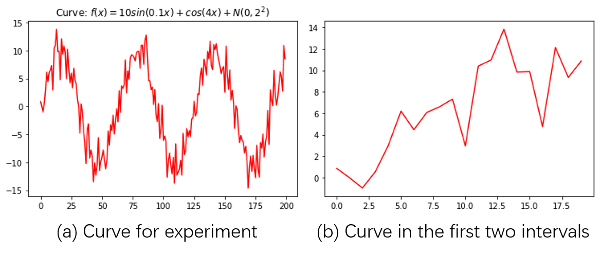
(a) is the whole plot, and (b) zooms in $[0,20]$.
For simplication, I use sample rate $1$ to sample interval $[0,200]$, forming $\pmb{x} = x[0],x[2],…,x[199]$. Notice that in this section, Python-styled $0-based$ indexing is used, for easy link with codes.
Configurations
Before implementing the algorithms, the whole problem still needs more specific definition: what is the hop length and the interval size?
When I am talking about hop length, I assumed that the sampling strategy is equal-stepped. In the this experiment, data points are equally sampled.
If we denote hop length as $\Delta_h i$ and interval size as $\Delta_I$, and each index interval as $I_i$, then: $I_i[0]+\Delta_h=I_{i+1}[0]$ and $I_i[-1]-I_i[0]=\Delta_I$. For example, the first index interval is $I_0 =[0,1,…,\Delta_I - 1] = [0:0+\Delta_I]$, the second index interval is $I_1 = [\Delta_h:\Delta_h+\Delta_I]$, and the third index interval is $I_2 = [2\Delta_h:2\Delta_h+\Delta_I]$, and so forth.
Because we can use a for-loop to implement LUC for each interval, let’s just focus on implementing LUC in one interval. When it comes to one interval, then its LP, candidate set and candidate pairs come into use. In this experiment, I compared four algorithms, which are:
- (LP-based) normal LUC algorithm, as introduced by Definition 1
- (LP-based) (non-full) candidate-set algorithm
- (LP-based) full candidate-set algorithm
- accompany-pair algorithm
I used SciPy to implement LP-based methods by calling the scipy linprog method.
One of the problems is to translate the LUC problem into the standard LP problem. The proof for Lemma 2 has already shown how to achieve this.
Another problem is to choose a proper method for LP solution. I tried different methods and concluded that the revised simplex method is most efficient.
For (non-full) candidate-set algorithm, I applied Algorithm 1,2,3,4 to find the candidate set, and then use LP (whose constraints are based on the candidate set) to find the solutions.
The full-candidate-set algorithm modifies the candidate-set algorithm by replacing Algorithm 3 with Algorithm 3.2.
For the accompany-pair algorithm, I apply Algorithm 5 only, which takes the role of LP.
LUC Results
In this experiment, I set $\Delta_h = 10$ and $\Delta_I = 10$.
First I extract the first two intervals and do LUC for them. Here is the result: 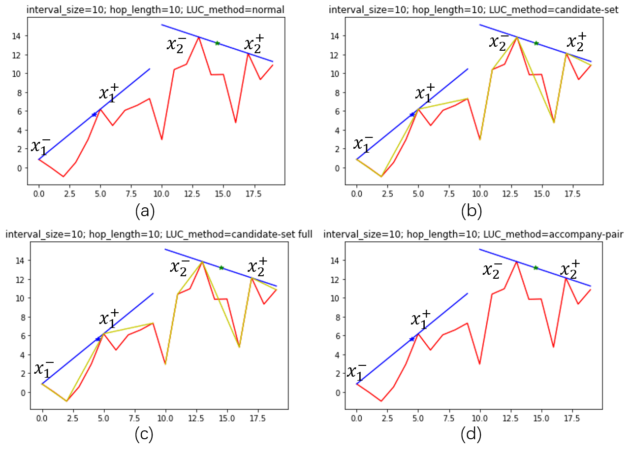 The yellow lines indicate candidate-sets, while the red lines indicate the original curve.
Those results verify the correctness of Lemma 2 by showing that at least two zero-slackness constraints are reached. They also show that applying full definition of candidate set does not lead to seriously different results compared with the results obtained by the non-full definition.
Then, I test the whole curve, which is shown in the following figure: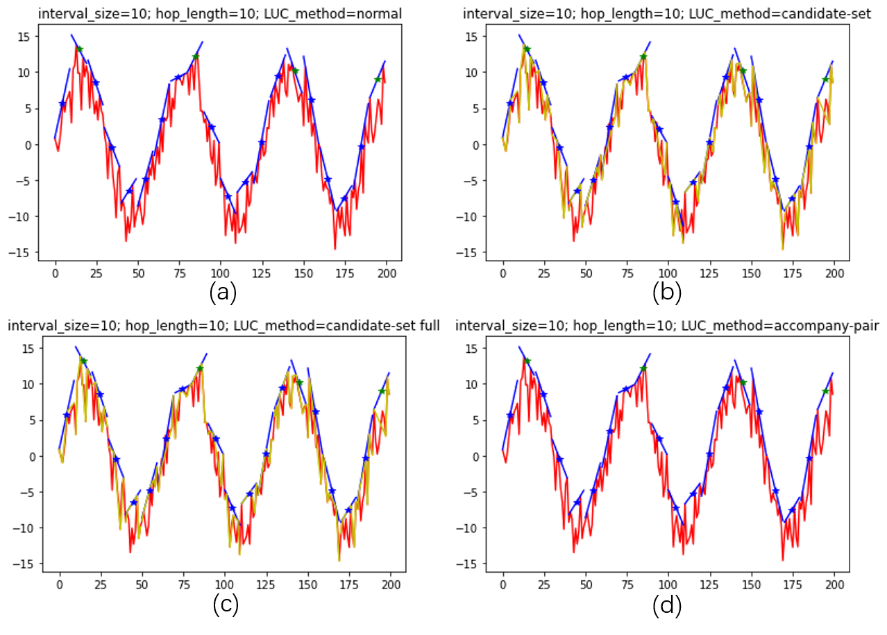 The green-star marks indicate local maxima of the centroid sequence, which are marked mostly by blue marks.
From the whole-curve result we can see several phenomena:
- The accompany-pair algorithm result is the same as the normal-LP algorithm result and the candidate-set-full algorithm result.
- There are slight differences between results of the candidate-set-full algorithm and non-full candidate-set algorithm.
- Peaks are correctly detected regardless of serious noise.
Phenomenon 1 verifies my Hypothesis 1 and 2, because the candidate-set-full algorithm and the accompany-pair algorithm is grounded on Hypothesis 1 and 2.
Phenomenon 2 gives us a hint that we can change candidate-set-full algorithm into non-full candidate-set algorithm without losing much accuracy. In the next section I will compare the time consumption between those two algorithms.
Phenomenon 3 verifies the effectiveness of LUC algorithm: after smoothed by LUC, it is OK to directly apply the strict $locmax$ function to the centroid serie and get the desired peaks.
Next, I will compare each algorithm more deeply regarding their time cost and correctness.
Time Consumption
For each algorithm, I adjusted interval size $\Delta_I$ and LP methods (except accompany-pair algorithm). I used Monte-Carlo method to reduce the variation of time cost estimation. In this test, I run each case for 100 times. Results are shown in the following figure: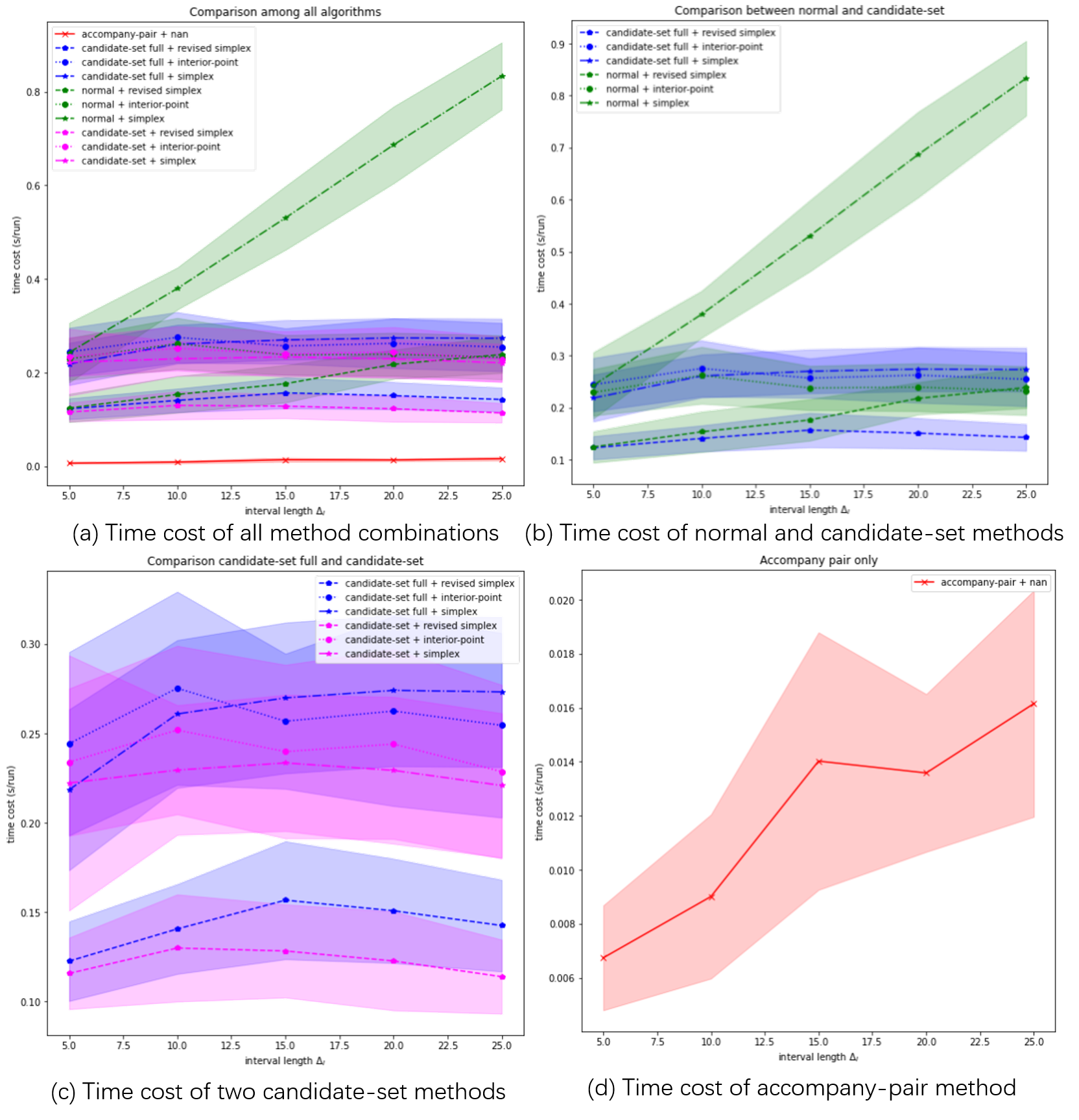 Time cost experiment results.
This experiment is done by my old laptop, whose CPU is an Intel CORE i5.
From the results, we can observe that:
- The most efficient algorithm is the accompany-pair algorithm, whose time cost is much lower than the others
- Candidate-set algorithm did reduce time cost compaired with normal algorithm, when the simplex-family LP methods are used. However, in when interior-point LP method is used, the candidate-set algorithm will be a little bit slower than normal algorithm.
- The revised simplex LP method is most efficient, while the original simplex LP method is least efficient.
- The full-candidate-set algorithm does not increase time cost too much compared with the non-full-candidate-set algorithm. Still, non-full-candidate-set algorithm is faster.
- The candidate-set algorithms show an interesting trend regarding $\Delta_I$: when $\Delta_I$ increases, time cost do not increase, but even decrease. This may be because that candidate-set filered out most irrelevant constraints and therefore there are less constraints left for LP.
Influence of SNR and SIR on LUC Accuracy
Influence of Interval Partition on LUC Accuracy
High-order LUC
It is not a must to apply $locmax$ directly after LUC. Insteac, we can do another LUC after LUC, which can be called as 2-order LUC. An example is shown in the following figure: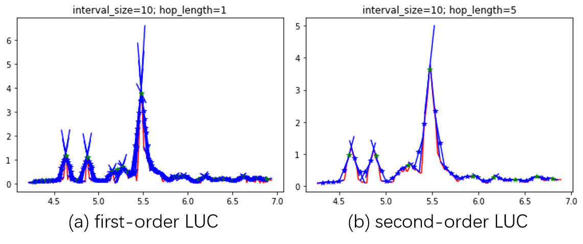
The first LUC, namely first-order LUC, adopts $\Delta_{h1}=1$ and $\Delta_{I1}=10$. This smoothifies the original curve, as shown in (a). The second-order LUC adopts $\Delta_{h2}=5$ and $\Delta_{I2}=10$, and then we get the correct peaks.
Notice that LUC is good at finding peaks with proper x-axis span. For example, in the figure above, the index width of each peak is around 20; when $\Delta_{h2}=5$, it is prone to find those peaks because 5 is around the same scale as 20, no matter how low those peaks are; when $\Delta_{h1}=1$, however, it is easier to find peaks of shorter x-axis span.
Experiment 2: LUC on Spectrograms
To demonstrate the potentials of LUC on audio analysis, I did another experiment, in which I applied LUC to find peaks in spectrograms.
A spectrogram consists of time-variant spectrums. Those spectrums may be FFT, CQT or mel-spectra etc. Normally, we use color to demonstrate the intensity at each time-frequency. An example of CQT spectrogram is shown as following: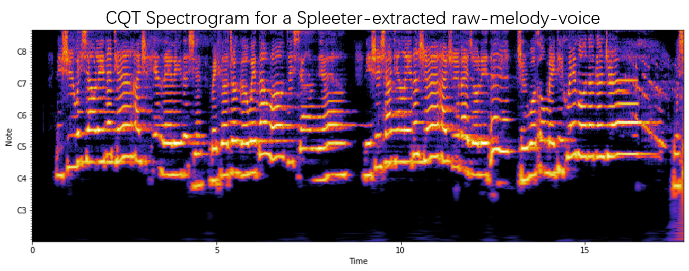
If those CQT stuff do not make sense to you, no need to worry. Just remember that our task is to find the peaks (bright stripes) in that spectrogram, ignoring noisy points.
Dealing with low-hight peaks
Sometimes, we do not want our model to detect low peaks, althought those peaks are wide enough. This leads to a problem: what exactly is our definition on a desired peak? On the one hand, we want a desired peak to be wide enough (otherwise, it is a fake peak); on the other hand, we want to ignore the peaks which are too low compared with the higher peaks. The first condition can be guarenteed by LUC, but LUC does not provide solution to meet the second condition. An example is shown in the following figure: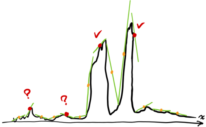
Therefore, we have to come up with a new way to discriminate those low peaks from high peaks. My solution is to weight the peaks with salience.
If a spectrogram $\pmb{S}=[s_{ft}]{F\times T}$ is inputted to a 1-order LUC, I hope my model can output a peak-weight map $\pmb{W}=[w{it}]_{L\times T}$. The relationship between $\pmb{S}$ and $\pmb{W}$ is as such:
- If hop length is $\Delta_h$ and interval size is $\Delta_I$, then $L=floor(\frac{F+\Delta_h-\Delta_I}{\Delta_h})$
- $w_{i}$ refers to the weights at the $i^{th}$ interval centroid.
Experiment 3: Comparing LUC with Existing Smoothing Methods
There are all kinds of existing smoothing methods, among which the most common ones include: low-pass filtering, kernel smoothing, moving average smoothing and local regression.
In order to fairly compare those methods, I use the same pipeline: signal → smoothing (to be tested) → locmax.
本文作者: lucainiaoge
本文链接: https://lucainiaoge.github.io.git/2020/10/10/linear-upper-coverage-algorithm-for-peak-finding/
版权声明: 本作品采用 Creative Commons authorship - noncommercial use - same way sharing 4.0 international license agreement 进行许可。转载请注明出处!
