
Intuition for Statistical Inference
by lucainiaoge
Intro
In a word, statistical inference deal with the problem of “trying to reach the God”. In other words, we observe data, and we try to fit to the distribution of such data. A little bit hard to understand? Hope that this article can help you understand that…
- An example: pictures
Suppose you are studying digital pictures $x \in \pmb{R^{M\times M}}$. Accordingly, its distribution is $p_G(x): \pmb{X_{G}} \rightarrow \pmb{R^+}\cup\pmb{O}$. One of our goals is to find exactly the subspace $\pmb{X_{G}}\subseteq\pmb{R^{M\times M}}$ where the pictures $x \in \pmb{X_{G}}$ look like hand-written numbers (correspondingly, $\pmb{X_{G}}$ is the space where the ${M\times M}$ hand-written number pictures are defined). Again, our mission is to find the $p_G(x): \pmb{X_{G}} \rightarrow \pmb{R^+}\cup\pmb{O}$ given a hand-written number dataset $\pmb{X_{s}}$.
We take $\pmb{X_{G}}$ as the “God/Ground-truth dataset” and $\pmb{X_{s}} \subseteq \pmb{X_{G}}$ as the “observation dataset” (e.g. MNIST).
Now, question is: how to fit to that God/Ground-truth distribution? Well… For each question, we have to represent it before we solve it. In this article, I try to represent it clearly.
This article does not try to solve those questions explicitly. The aim of this article is to remind you what you are really doing when you get lost in some annoying math works.
By the way, why it is important to estimate $p_G(\pmb{x})$? Because once we know $p_G(\pmb{x})$, we can do such things: 1. to judge whether a given data point $x_0$ belongs to our distribution $p_G(\pmb{x})$, and then we can do classification; 2. to sample data points according to $p_G(\pmb{x})$, and then we can do generation!
The Variational Problem
We have already been familiar with this form: given a vector space $X$ (e.g. $X=\lbrace 0,1,2 \rbrace$) and a function $f$ (e.g. $f(x)=x^2$), we want to solve
$$\mathrm{argmax}_{x∈X} f(x)$$
What about the argmax problem which finds the optimum function? i.e. given a function space $\mathcal{F}$ (e.g. $\mathcal{F}=\lbrace f: f(x)=x^2+c,c\in \pmb{R} \rbrace$) and a functional $F: \mathcal{F}→\pmb{R}$ (e.g. $F[f]=\int_0^1 f^2(x)dx$), we want to calculate:
$$\mathrm{argmin}_{f∈\mathcal{F}} F[f]$$
This problem is called a variational problem, which aims to find a function $f∈\mathcal{F}$ which minimizes/maximizes a functional $F$.
We have already encountered this kind of problem in information theory!
For example, we have already found the “discrete maximum entropy”
$$\mathrm{argmax}_{p∈\mathcal{P}} H[p]$$
If $\mathcal{P}= \lbrace AllDiscreteDistributionsWith\quad M \quad Values \rbrace$, and $H[p(x)]=\sum_{x}p(x) \mathrm{log} \frac{1}{p(x)}$, then
$$\mathrm{argmax}_{p∈\mathcal{P}} H[p]=U(x)$$
where, $U(x)$ is the uniform distribution on $M$ possible discrete values.
The Statistical Inference Variational Problem
Problem definitions
What we want to do is: given data $\pmb{x}$, we want to approximate its distribution $p_G(\pmb{x})$. i.e. we want to solve this variational problem:
$$p^*(\pmb{x})=\mathrm{argmax}_{p∈\mathcal{F}} D[p(\pmb{x}),p_G (\pmb{x})]$$
The term $p_G (\pmb{x})$ means the God’s distribution of data $\pmb{x}$, or the “Ground truth distribution”. Well, I have to say that we assumed that there is a ground truth (or GOD!), which is our philosophical point of view.
Now is the problem:
- Problem 1: How to define the functional (distance between distributions) $D[p(\pmb{x}),p_G (\pmb{x})]$?
- Problem 2: How to define the function space $\mathcal{F}$?
Problem 1: where the “Maximum Likelihood” comes from
Problem 1: how to find the functional (distance between distributions) $D[p(\pmb{x}),p_G (\pmb{x})]$? Note that we do not know the GOD distribution i.e. $p_G(\pmb{x})$. Thus, it is impossible to calculate this functional by directly calculating the distance between $p(\pmb{x})$ and GOD distribution. However, there is an easy way to define $D[p(\pmb{x}),p_G (\pmb{x})]$ as:
$$D[p(\pmb{x}),p_G (\pmb{x})]≜\mathrm{log}p(\pmb{x})$$(Other ways include estimating the momentums or other sufficient statistics. Those are out of the current scope.)
For i.i.d. data $\pmb{x}$, we can even write $\mathrm{log}p(\pmb{x})$ as $\mathrm{log}p(\pmb{x})=\sum_{i=1}^N \mathrm{log}p(x_i)$
The term $\mathrm{log}p(\pmb{x})$ is called as “log-likelihood”, and the variational problem $p^*(\pmb{x})=\mathrm{argmax}_{p∈\mathcal{F}} D[p(\pmb{x}),p_G (\pmb{x})]$ is called “maximum likelihood”, which we have already been familiar with.
(Note that in the scheme of “maximum likelihood”, we did not consider $p_G (\pmb{x})$ explicitly. We assumed that if $\pmb{x}$ is from the ground-truth, $p_G (\pmb{x})$ should always be larger or equal than other $p(\pmb{x})$. We tend to think that “what we see is GOD”. Or in other words, “data (what we observed) are all we know, and we cannot do better unless we know more information (more data, or more observations)”. The “momentum estimation method” directly applies this philosophical assumption, i.e. calculating the distances between moments in order to make $p(\pmb{x})$ as near as $p_G (\pmb{x})$.)
Problem 2: to parameterize or not to
Well… For problem 2, we have two ways: to parameterize or not.
What is parameterization? I use an example to illustrate that:
Suppose the data $\pmb{x}$ are 1D. And we assume the function space is Gaussian, i.e. $\mathcal{F}=\lbrace AllOneDimGaussianPDFs \rbrace$. We can easily write $\mathcal{F}$ in the form of the space of its sufficient statistics (i.e. $\mu$ and $\sigma$). In other words, the space $\Theta=\pmb{R}\times\pmb{R^+}$ is actually the function space $\mathcal{F}$. And there exists a unique Gaussian Function $G:\Theta→\mathcal{F}$ such that for any $(\mu,\sigma)∈\Theta$, $G(\mu,\sigma)=f(x\vert \mu,\sigma)∈\mathcal{F}$
In this case, we parameterized $\mathcal{F}$ with $\Theta$, with the distribution assumption $P:\Theta→\mathcal{F}$. In other words, $\Theta$ are the parameters which control the function space. Thus, the variational problem
$$p^*(\pmb{x})=\mathrm{argmax}_{p∈\mathcal{F}} D[p(\pmb{x}),p_G (\pmb{x})]$$
can be written as an argmax problem for parameters:
$$\theta^*=\mathrm{argmax}_{\theta∈\Theta} D[f(\pmb{x}\vert\theta),p_G (\pmb{x})]$$
$$p^* (\pmb{x})=P(\theta^* )$$
Of course, we can search the $\mathcal{F}$ directly without introducing $\Theta$ and $P:\Theta→\mathcal{F}$. How to search $\mathcal{F}$ given $\pmb{x}$? There are also various ways (e.g. $k-means$). However, we are not talking about those methods right now.
A statement for a challenge: how to find the God - bias vs. variance
How to assume a nice function space $\mathcal{F}$ such that the $p^* (\pmb{x})∈\mathcal{F}$ is easy to find and that $D[p(\pmb{x}),p_G (\pmb{x})]$ is relatively small? In other words, the function space $\mathcal{F}$ (or parameter space $\Theta$ in the case of parameterization) should satisfy such properties in order to be a good one:
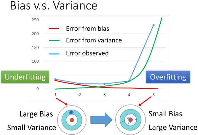
- there exists $p^* (\pmb{x}))∈\mathcal{F}$ such that $D[p(\pmb{x}),p_G (\pmb{x})]$ is small, i.e. $\mathrm{E}_{\pmb{x}\in\pmb{X_G}} [D[p(\pmb{x}),p_G (\pmb{x})]]$ is small;
- $D[p(\pmb{x}),p_G (\pmb{x})]$ cannot be too unstable, i.e. $\mathrm{Var}_{\pmb{x}\in\pmb{X_G}} [D[p(\pmb{x}),p_G (\pmb{x})]]$ is small.
If $\mathrm{E}_{\pmb{x}\in\pmb{X_G}} [D[p(\pmb{x}),p_G (\pmb{x})]]$ is small, we say that the function space F is of small bias compared with the GOD’s function $p_G (\pmb{x})$;
If $\mathrm{Var}_{\pmb{x}\in\pmb{X_G}} [D[p(\pmb{x}),p_G (\pmb{x})]]$ is small, we say that the function space $\mathcal{F}$ is of small variance compared with the GOD’s function $p_G (\pmb{x})$, or that our model $p^* (\pmb{x})$ has a good ability to generalize. The term “generalize” means that no matter what data $\pmb{x}$ is given, the difference between $p^* (\pmb{x})$ and $p_G (\pmb{x})$ will not change too much.
Intuition from Hung-yi Lee: see the pictures in
http://speech.ee.ntu.edu.tw/~tlkagk/courses/ML_2016/Lecture/Bias%20and%20Variance%20(v2).pdf
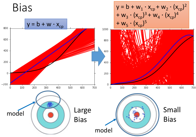
Each “sample point $p_s^* (\pmb{x})$” is actually an instance of $p_s^*(\pmb{x})=\mathrm{argmax}_{p∈\mathcal{F}} D[p(\pmb{x}),p_G (\pmb{x})]$, where $\pmb{x}\in\pmb{X_s}$, and $\pmb{X_s}$ (e.g. MNIST) is a subset of the God data set $X_G$ (e.g. all possible pictures of handwritten numbers).
Afterwards…
You have already got an intuition of our challenges. Now, time to solve the challenges! Of course, for several specific problems, simple models are enough! For example, if we want to fit a Gaussian distribution, the most convenient way is to calculate the mean and variance of the dataset (observation). However, most problems are complex in reality. We have to design models which can deal with such complexity.
A genious way is to introduce Latent Variables to make our models more powerful. We assume that the Latent Variables can reveal the underlying modes of our observations. How to calculate the Latent Variables and find the argmax? We will discuss later when introducing HMM (Hidden Markov Model), GMM (Gaussian Mixure Model), EM (Expectation Maximization) algorithm and variational inference. The Latent Variable trick is in fact a statistical assumption.
Another genious way is to use Neural Networks in order to fit arbitrary functions. The Neural Networks trick is in fact a structural (connectivism) assumption.
In order to reduce the variance, more tricks can be considered (e.g. early stopping, dropout, normalization, residual connection, parameter sharing, simplified models…). Details are overwhelming. Not going to introduce them here!
本文作者: lucainiaoge
本文链接: https://lucainiaoge.github.io.git/2020/08/03/intuition-for-statistical-inference/
版权声明: 本作品采用 Creative Commons authorship - noncommercial use - same way sharing 4.0 international license agreement 进行许可。转载请注明出处!
